NHC
An Evaluation of NHC Service Enhancements, Part 2: Post-Tropical Cyclone Advisories
Brad Reinhart, Hurricane Specialist
In Part 1 of this blog series, we discussed the NHC’s usage of Potential Tropical Cyclone advisories to better message the threats posed by tropical cyclones (TCs) that develop near land. Another challenging situation occurs when a tropical cyclone loses its tropical characteristics while it approaches the coastline. For example, Sandy (2012) lost its tropical characteristics and transitioned into a post-tropical cyclone near the time of landfall, which made communicating hazard information difficult. Following that event, the National Weather Service (NWS) adopted a policy to improve service during similar future situations. Under current policy, if the post-tropical cyclone poses a significant threat to life and property, and if the transfer of responsibility to another NWS office1 would result in a discontinuity in service, the NHC will continue to write advisories on the system. This includes the full suite of standard TC products, watches, warnings, and hazard information.
This policy change was driven by a desire to ensure consistent product availability and messaging during high-impact events. Has it worked? Let’s take a closer look at how NHC has leveraged this strategy in recent hurricane seasons.
What Is a Post-Tropical Cyclone?
Post-tropical cyclone is a generic term for a system that was formerly a TC, but no longer possesses sufficient tropical characteristics to be classified as a TC. As a reminder, TCs are warm-core and non-frontal cyclones with organized deep convection and a closed surface wind circulation about a well-defined center. In the Atlantic Ocean, TCs commonly transition to extratropical (ET) cyclones as they recurve into the mid-latitudes. Since an ET cyclone derives its energy from temperature differences between warm and cold air masses and is associated with fronts, its structure is fundamentally different from a TC. So once a weather system transitions to an ET cyclone, it no longer satisfies TC criteria and would be considered “post-tropical”.

A common misconception is that a TC has been “downgraded” when it becomes a post-tropical cyclone. This is certainly not the case. Unlike systems in their developmental stages that tend to be weaker before genesis, many post-tropical cyclones are powerful systems that simply no longer possess tropical characteristics. An analysis of NHC post-tropical cyclone advisory events (below) indicates that over half of these cyclones were producing winds of 58 mph or greater at the time of post-tropical transition. Four of these systems were producing hurricane-force (≥ 74 mph) winds when they became post-tropical cyclones. In addition to strong winds, these systems can produce other hazards that pose a significant threat to life and property on land. Storm surge, destructive waves, and flooding rains are dangerous regardless of whether the system producing these conditions is still a TC or has recently become a post-tropical cyclone. Furthermore, ET cyclones often have a larger wind field than TCs, which increases the footprint of potential wind and surge impacts.

Usage of Post-Tropical Cyclone Advisories

From 2013-2022, the NHC has issued 41 advisories for 13 Atlantic post-tropical cyclones. The figure below shows the length of time that NHC continued to provide forecasts for each storm following its post-tropical transition. While the majority of the post-tropical cyclone advisories lasted for 12 hours or less, a few events continued for longer than 24 hours. In 2016, the NHC issued advisories for an additional three days as Post-Tropical Cyclone Hermine meandered offshore the U.S. Mid-Atlantic coast.

The table below provides a summary of how often different watches and warnings were in effect with post-tropical cyclone advisories. While tropical storm warnings are most commonly in effect, there have been a couple of instances where hurricane and storm surge warnings were maintained with post-tropical cyclone advisories. This strategy is used not only for United States land threats, but international ones as well. Because many Atlantic TCs become ET cyclones as they recurve northward over the western Atlantic Ocean, some post-tropical cyclones bring significant impacts to Atlantic Canada as they pass near or over the region. The Canadian Hurricane Centre (CHC) has issued Tropical Storm and Hurricane Watches and Warnings for tropical and post-tropical cyclones since 2004, so the NHC policy aligns well with our colleagues in Canada. As we will show, this consistency has resulted in more effective hazard communication for post-tropical cyclones that have impacted Canada in recent years.

Case Studies
Hurricane Matthew (2016)

Matthew was a catastrophic storm that made landfall in Haiti as a category 4 hurricane (on the Saffir-Simpson Hurricane Wind Scale), resulting in hundreds of fatalities and widespread damage. After additional major hurricane landfalls in Cuba and the Bahamas, Matthew moved roughly parallel to the coast of the southeastern United States and made a final hurricane landfall in South Carolina. As Matthew moved back offshore and passed near the North Carolina coast, the cyclone began losing tropical characteristics as it interacted with an approaching frontal system and became a 75-mph extratropical cyclone while it was centered about 60 miles east of Cape Hatteras, North Carolina.
Although no longer a hurricane, Matthew was still producing very strong winds to the west of its center, resulting in hurricane-force gusts over coastal portions of eastern North Carolina and a continued storm surge on the sound side of the barrier islands. Due to these continued land impacts, the NHC retained advisories on Post-Tropical Cyclone Matthew and maintained Tropical Storm Warnings and Hurricane Watches for portions of coastal North Carolina, as well as for the Pamlico and Albemarle sounds. (Note: The NWS did not introduce an operational storm surge watch/warning until 2017). The NHC produced a couple of extra advisories until the post-tropical cyclone moved far enough offshore that the wind and surge threat subsided for coastal North Carolina. Ultimately, the highest coastal water levels in the state occurred on the sound side of the Outer Banks, with maximum estimated inundation levels of 4-6 feet above ground level. Although significant storm surge and freshwater flooding was reported on some of the barrier islands, property damage from flooding and high winds was generally minor.

Hurricane Dorian (2019)
Most people remember Dorian for the extreme devastation it caused as the strongest hurricane to hit the northwestern Bahamas in modern recorded history. However, the hurricane also affected a large portion of the U.S. East Coast as it recurved and passed over the western Atlantic Ocean. On its approach to Atlantic Canada, Dorian lost its tropical characteristics and transitioned to a 90-mph post-tropical low. Given Dorian’s significant threat to life and property, the NHC, in coordination with the CHC, decided to continue issuing advisories on the post-tropical cyclone as it neared the Canadian Maritimes. The CHC maintained Hurricane Warnings that were in effect for portions of Atlantic Canada. The NHC Key Messages stressed the significant impacts expected from significant storm surge and hurricane-force winds. Overall, the NHC provided an extra 30 hours of advisories that covered Post-Tropical Cyclone Dorian’s trek across eastern Canada.
As a post-tropical cyclone, Dorian produced extensive wind damage over portions of the Canadian Maritimes, including downed trees and power lines along with roof and siding damage. Heavy rainfall resulted in major flooding, and storm surge accompanied by large waves caused significant coastal erosion. Insurance estimates indicate that Dorian caused over $75 million (USD) in damage across Atlantic Canada.
Hurricane Fiona (2022)


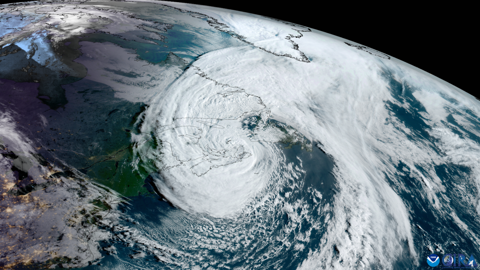
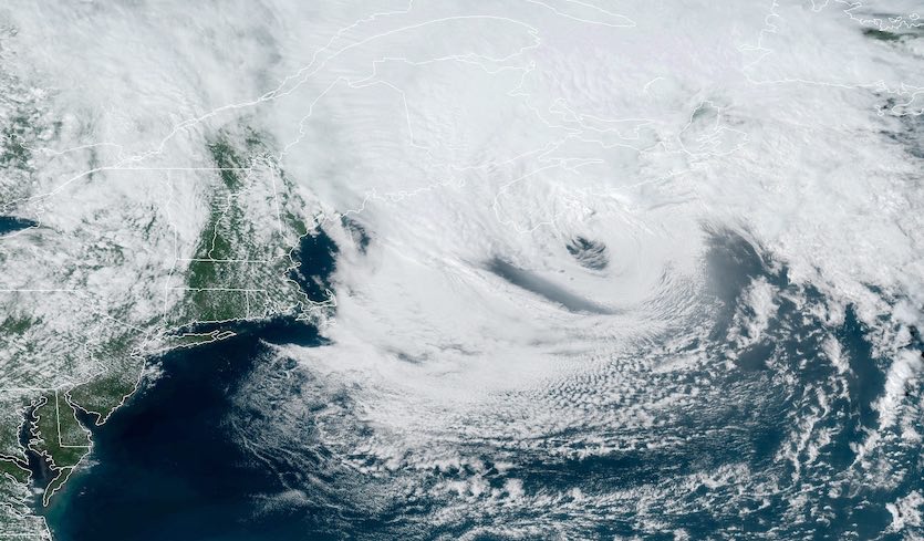
GOES-16 combined visible and infrared satellite images of Fiona on September 22, 2022 at 1800 UTC as a major category 4 hurricane (left), and September 23, 2022 at 1800 UTC shortly before it transitioned to a post-tropical cyclone (right).
Hurricane Fiona made landfall in Guadeloupe, Puerto Rico, the Dominican Republic, and Grand Turk before it turned north-northeastward over the western Atlantic ahead of an approaching frontal system. As the tropical cyclone interacted with the associated mid- to upper-level trough, Fiona lost its tropical characteristics and accelerated toward Atlantic Canada. Due to the significant threat of high winds, storm surge, and large waves that the storm posed to Atlantic Canada, the NHC continued to produce advisories on Fiona and the CHC maintained the Hurricane Warnings in effect. Fiona became an intense 115-mph post-tropical/extratropical cyclone shortly before it reached the coast of Nova Scotia, and it made landfall as the deepest cyclone (by minimum pressure) on record in Canada with maximum sustained winds of 100 mph. Ultimately, the NHC provided an additional 18 hours of advisories on Post-Tropical Cyclone Fiona until the tropical storm and hurricane warnings were discontinued.
Fiona produced devastating impacts across Atlantic Canada as a post-tropical cyclone. Storm surge and large, destructive waves resulted in devastating coastal flooding and significant erosion along the coasts of southwestern Newfoundland, eastern and northern Nova Scotia, Prince Edward Island, eastern New Brunswick, and Iles-de-la-Madeleine. Two people drowned, and over 100 homes were destroyed along the coast of southwestern Newfoundland from Port aux Basques eastward to Burgeo. Elsewhere, strong winds downed thousands of trees and power lines across portions of Nova Scotia, New Brunswick, Prince Edward Island, and Newfoundland. Catastrophe Indices and Quantification Inc. (CatIQ) damage estimates indicate that Fiona is the costliest extreme weather event on record in Atlantic Canada with about $800 million (CAD) in insured losses.
“In some ways, Fiona was Canada’s version of Sandy – a landmark event,” according to Chris Fogarty, Program Manager at the Canadian Hurricane Centre. “Impacts were forecast to be considerable, and the CHC focused on the impacts in the warning statements even after the storm was declared post-tropical.”

Conclusion
The NHC service enhancements discussed in this blog series were the direct result of lessons learned from past events. Sandy was a unique storm that exposed hazard communication and messaging challenges that can arise when a TC becomes post-tropical around the time of landfall. In response, the NWS adopted a policy that attempts to keep the public focus on the warnings and potential impacts of the storm, regardless of its status. Ultimately, our ability to issue full NHC advisory packages on post-tropical cyclones has been successfully utilized in recent years, both domestically and internationally. The examples presented here serve as reminders that post-tropical cyclones can bring significant impacts to land areas, and the associated warnings must be taken seriously.
Footnotes
1 After NHC discontinues advisories, post-tropical cyclones that do not pose a threat to land areas are discussed in High Seas Forecasts issued by NHC’s Tropical Analysis and Forecast Branch (TAFB) and/or the NOAA Ocean Prediction Center (OPC). If an inland system still poses a threat of heavy rains and flash floods in the United States, advisory responsibility is transferred to the NOAA Weather Prediction Center (WPC) until the flash flood threat has ended.
Share this:

An Evaluation of NHC Service Enhancements, Part 1: Potential Tropical Cyclone Advisories
Brad Reinhart, Hurricane Specialist

Tropical cyclone (TC) formation near land is among the more difficult scenarios for forecasters, emergency managers, and the general public to contend with during the hurricane season. In the past, these situations were challenging from a public warning and hazard communication perspective because tropical storm and/or hurricane watches and warnings could only be issued once TC formation occurred. However, National Weather Service (NWS) policy changes in 2017 gave the National Hurricane Center (NHC) the ability to issue Potential Tropical Cyclone (PTC) advisories. These advisories can be initiated when a disturbance is not yet a TC, but poses a threat of becoming a TC and bringing tropical storm or hurricane conditions to land areas within 48 hours. So instead of sacrificing valuable lead time by waiting until TC formation occurs, the NHC can issue the full suite of advisory products (including tropical storm, hurricane, and storm surge watches and warnings) for near-term land threats before genesis occurs.
How often has the NHC employed this strategy? Have PTC advisories improved our ability to effectively warn people in advance of hazardous events? Let’s take a closer look at how PTC advisories have been used in recent hurricane seasons.
Forecaster Considerations
When deciding to initiate PTC advisories, hurricane specialists must weigh several factors. The primary consideration is the likelihood of tropical storm or hurricane-force winds occurring on land within the next 48 hours. If the system is over open waters and does not pose a near-term land threat, PTC advisories will not be issued and potential hazards for marine interests will be covered by marine products and warnings. The disturbance should have a “trackable” cloud system center that allows for some measure of forecast continuity. If the system is so disorganized that a system center cannot be identified, it will be very difficult to issue accurate and consistent pre-genesis forecasts. Another consideration is the disturbance’s potential for tropical cyclone development. Although the issuance of PTC advisories is not directly tied to a system’s formation chance in the Tropical Weather Outlook (TWO), it makes sense that the NHC would only start PTC advisories for systems that they are reasonably confident will become tropical cyclones, as too many false alarms could reduce the long-term effectiveness of our watches and warnings. The scatterplot below shows the 2-day and 5-day1 TWO genesis probabilities at the issuance time of the initial PTC advisory for each system. Note that the size of the marker indicates the frequency of occurrence for a particular pair of 2-day/5-day chances. The 2-day and 5-day TWO formation chances at the initial PTC advisory time all range from 70-100%, which is within the “high” category of the TWO. Most commonly, these disturbances have 2-day formation chances of 80-90% when PTC advisories are initiated, which indicates very high confidence in the near-term formation potential.

Usage of Potential Tropical Cyclone Advisories
From 2017-2022, the NHC issued 116 potential tropical cyclone advisories for 30 different systems – 27 in the Atlantic Ocean and 3 in the eastern North Pacific Ocean (map below). Of the 30 total PTC cases, only three disturbances failed to develop into tropical cyclones. At least three Atlantic PTC cases have occurred each year since 2017. During the 2022 season, PTC advisories were used for five Atlantic disturbances, four of which went on to become tropical cyclones – Alex, Bonnie, Julia, and Lisa.

While the majority of PTC disturbances were producing maximum sustained winds below tropical storm force (30-35 mph) when advisories were initiated, 20% of PTCs were already at tropical storm intensity for the first advisory. These cases were often fast-moving and/or sheared systems that lacked a closed surface circulation and/or enough convective organization to be officially classified as a TC.

The table below provides a summary of how often different watches and warnings were issued with PTC advisories. While tropical storm watches and warnings are most commonly issued with PTC advisories, there have been several instances of hurricane and storm surge watches being issued as well. Additionally, a storm surge warning was issued with a PTC advisory for the system that became Tropical Storm Nestor in 2019. The PTC advisories have been used to issue watches and warnings for both the United States and international locations. In fact, 80% of PTC events have resulted in the issuance of a watch or warning internationally, while 37% have resulted in watch or warning issuance for the United States and its Caribbean territories (Puerto Rico and the U.S. Virgin Islands).

The chart below illustrates the time difference between the issuance of the first PTC advisory for individual systems and the operational designation of those systems as TCs. This is one way to visualize how much earlier forecast and warning information was provided for these developing systems that posed a threat to land. On average, PTC advisories were initiated 18-21 hours before a system was operationally classified as a TC. However, there were a couple of 2022 storms (Bonnie and Alex) where PTC advisories were issued 88 hours and 57 hours, respectively, before genesis occurred. In these situations, the timing of genesis was challenging to forecast and ultimately occurred much later than expected. We will take a closer look at the Alex case later.

Warning Lead Times
We can also examine the lead time for warnings that have been issued with PTC advisories. Here, the lead time is defined as the time between warning issuance and the onset of sustained tropical-storm-force winds on land within the warning area, as determined during post-analysis and detailed in our Tropical Cyclone Reports. For this analysis, we looked at verified Tropical Storm Warnings that were issued with PTC advisories for the United States (including Puerto Rico and the U.S. Virgin Islands). International locations were not included because although NHC makes international watch and warning recommendations, the final decision is made by the national meteorological service or government of the respective countries.
The blue bars represent the actual lead times that were achieved using PTC advisories, while the red bars show the hypothetical lead times if warnings had not been issued until the disturbance became a TC. On average, verified Tropical Storm Warnings that were issued with PTC advisories provided an additional 21 hours of lead time than if PTC advisories had not been used. Sometimes, warnings issued with PTCs provided even more advanced notice. In 2020, a Tropical Storm Warning was issued for Puerto Rico and the U.S. Virgin Islands as the disturbance that became Isaias approached the Lesser Antilles. Although Isaias did not become a tropical storm until it passed south of Puerto Rico, the warning issued with the first PTC advisory provided about 45 hours of lead time before sustained tropical-storm-force winds reached the island.

Case Studies
Hurricane Barry (2019)


GOES-16 true color visible imagery of (left) Potential Tropical Cyclone Two at 1500 UTC July 10, 2019, and (right) Hurricane Barry making landfall at 1500 UTC July 13, 2019.
Barry originated from a non-tropical, mesoscale convective complex that emerged over the northeastern Gulf of Mexico on July 9, 2019. The elongated low pressure system was forecast to acquire tropical characteristics and strengthen over the northern Gulf of Mexico, and the NHC initiated PTC advisories at 10:00 am CDT on July 10 to issue Storm Surge and Tropical Storm Watches for portions of the Louisiana coast. Six hours later, a Hurricane Watch was issued for portions of Louisiana while the disturbance was still classified as a PTC. The disturbance developed into Tropical Storm Barry 24 hours after the first PTC advisory, and it ultimately strengthened into a hurricane shortly before landfall. The usage of PTC advisories allowed the NHC to issue the watches 48 hours before the onset of sustained tropical-storm-force winds along the Louisiana coast. Barry produced $600 million in damage according to NOAA National Centers for Environmental Information (NCEI), primarily in Louisiana due to flooding from heavy rains and storm surge.
Tropical Storm Claudette (2021)


GOES-16 true color visible imagery of (left) Potential Tropical Cyclone Three at 2100 UTC June 17, 2021, and (right) Tropical Storm Claudette making landfall at 0900 UTC June 19, 2021.
Claudette developed from a broad low-pressure system that formed over the southwestern Gulf of Mexico on June 14, 2021. The low meandered over the next couple of days before moving generally northward toward the northern Gulf Coast, but it did not possess a well-defined center or enough organized convection to be classified as a tropical storm. The NHC initiated PTC advisories at 4:00 pm CDT on June 17 to issue a Tropical Storm Warning for the northern Gulf Coast from Intracoastal City, Louisiana, to the Alabama/Florida border. The system remained sheared and somewhat elongated as its ill-defined center approached the Louisiana coastline, and operationally it was not designated Tropical Storm Claudette until early on June 19 when it made landfall along the coast of Terrebonne Parish, Louisiana. The Tropical Storm Warning was issued 21 hours before tropical-storm-force winds reached the Louisiana coast. Although this is less than the desired warning lead time of 36 hours, it is noteworthy because tropical storm conditions were already affecting the coast when Claudette operationally became a TC. Therefore, if the warning had been dependent on TC formation, there would have been no lead time at all! Claudette was responsible for four direct deaths in the United States, and NOAA NCEI estimates that the storm caused $375 million in damage from flooding, tornadoes, and gusty winds.
Potential Tropical Cyclone One / Tropical Storm Alex (2022)

On June 2, 2022, the NHC began issuing PTC advisories on a broad low-pressure area over the southern Gulf of Mexico near the Yucatan Peninsula. The system was forecast to move northeastward, gradually strengthen and become better organized, and eventually develop into a tropical storm before it moved across South Florida. This warranted the issuance of Tropical Storm Watches and Warnings for portions of western Cuba, the Florida Keys, and the Florida peninsula. But over the next couple of days, the center of the disturbance remained poorly defined, and the shower and thunderstorm activity failed to become more organized due to strong westerly vertical wind shear. As a result, the system did not become a TC before it reached the southwestern coast of Florida on the morning of June 4. In fact, the disturbance did not become Tropical Storm Alex until it crossed the Florida peninsula and moved over the southwestern Atlantic Ocean later that evening.
Although the disturbance was not a TC when it impacted Cuba and South Florida, the early NHC advisories heightened awareness and enhanced the messaging of a wind and flooding threat for these locations. The disturbance caused four flood-related fatalities in Cuba. Widespread flash and urban flooding, along with tropical-storm-force wind gusts, occurred across portions of South Florida, including the Miami metropolitan area. In this case, the status of the system as it impacted Florida was less important than the enhanced messaging that the NHC provided to the public through its use of PTC advisories.
Conclusion
The NHC has leveraged PTC advisories to address some of the challenges posed by TCs developing near land. This approach has maintained consistent hazard messaging during the developmental stages of TCs near land and increased watch and warning lead times to facilitate preparedness actions. The cases presented here are just a few examples of how the NHC has successfully used PTC advisories to provide better service to those who are threatened by these types of storms. Occasionally, there are still systems that undergo unlikely or unexpected genesis near the coast, resulting in short-fused warnings. However, the usage of PTC advisories and continued improvements in TC genesis forecasts should hopefully reduce these occurrences going forward.
Part 2 of this blog series will explore how the NHC has used advisories on post-tropical cyclones to maintain consistent warnings and hazard messaging for systems that are no longer officially classified as TCs, but continue to pose a significant land threat.
Footnotes
1 Beginning in 2023, NHC has extended the forecast time period covered by the TWO from 5 to 7 days. https://www.nhc.noaa.gov/pdf/NHC_New_Products_Updates_2023.pdf
Share this:

Was 2020 a Record-Breaking Hurricane Season? Yes, But. . .
Chris Landsea and Eric Blake [1]
An Incredibly Busy Hurricane Season
The 2020 Atlantic hurricane season was extremely active and destructive with 30 named storms. (The Hurricane Specialists here at the National Hurricane Center use the designation “named storms” to refer to tropical storms, subtropical storms, hurricanes, and major hurricanes.) We even reached into the Greek alphabet for names for just the second time ever. The United States was affected by a record 13 named storms (six of them directly impacted Louisiana), and a record yearly total of 7 billion-dollar tropical cyclone damage events was recorded by the National Centers for Environmental Information (https://www.ncdc.noaa.gov/billions/time-series/US). Nearly every country surrounding the Gulf of Mexico, Caribbean Sea, and tropical/subtropical North Atlantic was threatened or struck in 2020. Total damage in the United States was around $42 billion with over 240 lives lost in the United States and our neighboring countries in the Caribbean and Central America.

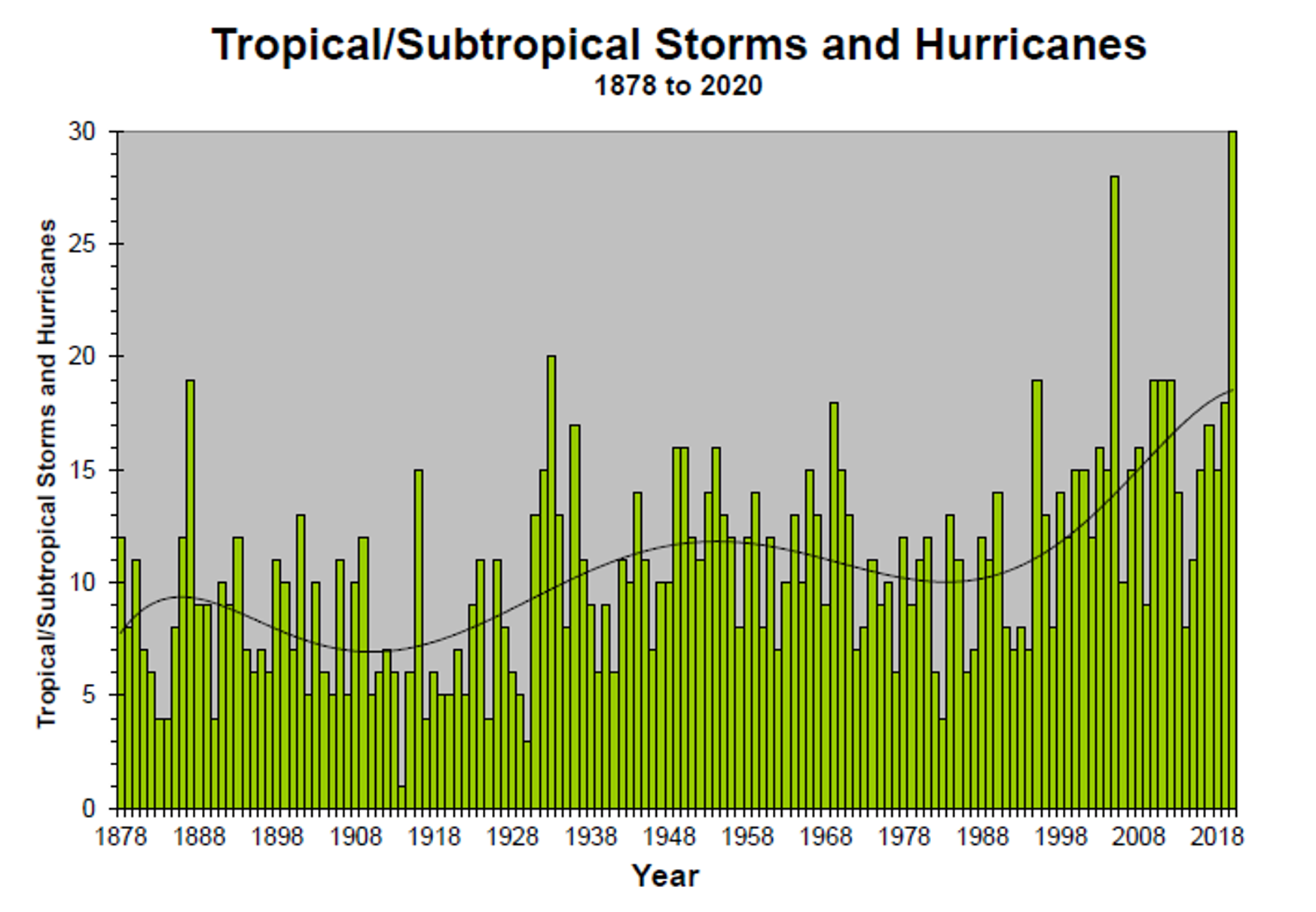
The 30 named storms in 2020 sets a record going back to the 1870s when the U.S. Signal Service (a predecessor to the National Weather Service) began tracking tropical storms and hurricanes. The only year that comes close is 2005 with 28 named storms. It’s also apparent that a very large increase has occurred in the number of observed named storms from an average of 7 to 10 a year in the late 1800s to an average of 15 to 18 a year in the last decade or so – a doubling in the observed numbers over a century! (The black curve in the figure below represents a smoothed representation of the data that filters out the year to year variability in order to focus on time scales of a decade or more).
However, the number of named storms is only one measure of the overall measure of a season’s activity. And indeed, for the 2020 season, other measures of Atlantic tropical storm and hurricane activity were not record breaking. For example, the number of hurricanes (14) was well above average, but fell short of the previous record of 15 hurricanes that occurred in 2005.
For overall monitoring of tropical storm and hurricane activity, tropical meteorologists prefer a metric that combines how strong the peak winds reached in a tropical cyclone, and how long they lasted – called Accumulated Cyclone Energy or ACE[2]. By this measure, 2020 was extremely busy, but not even close to record breaking. In fact, with a total ACE of 180 units, 2020 was only the 13th busiest season on record since 1878 with seasons like 1893, 1933, 1950, and 2005 substantially more active than 2020. One can also see that while there is a long-term increase in recorded ACE since the late 1800s, it’s quite a bit less dramatic than the increase seen with named storms. There also is a pronounced busier/quieter multi-decadal (40- to 60-year) cycle with active conditions in the 1870s to 1890s, late 1920s to 1960s, and again from the mid-1990s onward. Conversely, quiet conditions occurred in the 1900s to early 1920s and 1970s to early 1990s.

Technology Change and Named Storms
So why would the record for named storms be broken in 2020, while the overall activity as measured by ACE is not even be close to setting a record?
The answer is very likely technology change, rather than climate change. Today we have many advanced tools to help monitor tropical and subtropical cyclones across the entire Atlantic basin such as geostationary and low-earth orbiting satellite imagery, the Hurricane Hunter aircraft of the U.S. Air Force Reserve and National Oceanic and Atmospheric Administration (NOAA), coastal weather radars, and scatterometers (radars in space that provide surface wind measurements). In addition, the instrumentation and measuring techniques used by the satellites, aircraft and radars are continually improving. These technological advances allow us at the National Hurricane Center to better identify, track, and forecast tropical and subtropical cyclones with an accuracy and precision never before available. This is great news for coastal residents and mariners, since these tools help us provide the best possible forecasts and warnings to aid in the best preparedness for these life-threatening systems.
Such technology, though, was not available back at the advent of the U.S. Signal Service’s tropical monitoring in the 1870s. Without these sophisticated tools, meteorologists in earlier times not only had difficulty in forecasting tropical cyclones, but they also struggled in even knowing if a system existed over the open ocean. In the late 19th and early 20th Centuries, the only resource hurricane forecasters could use to monitor tropical cyclones were weather station observations provided via telegraph. Such an approach is problematic for observing – much less forecasting – tropical cyclones that develop and spend most of their lifecycle over the open ocean. Here’s a timeline of critical technologies that have dramatically improved tropical meteorologists’ ability to “see” and monitor tropical cyclones:

The upshot of all of these advances in the last century is much better identification of the existence of tropical cyclones and their strongest winds (or what meteorologists call “Intensity”). So, the further one goes back in time, the more tropical cyclones (and portions of their life cycle) were missed, even for systems that may have been a major hurricane. This holds for both counting named storms back in time as well as integrated measures like ACE. Our database is incomplete and has – as statisticians would say – a severe undersampling bias that is much more prominent earlier in the record. HURDAT2 – our Atlantic hurricane database – is an extremely helpful record which is a “by-product” of NHC’s forecasting operations, but it is very deficient for determining real long-term trends. (It’s important to point out that many data entries in HURDAT2 for intensity and even the position of the named storms are educated guesses as opposed to being based on observations before the 1970s advent of regular satellite imagery). To be able to examine questions about any impact from man-made global warming (aka climate change) on long-term changes in the number of named storms, for example, one must first account for the massive technology change over the last century.
Fortunately, to help address this issue, researchers at NOAA’s Geophysical Fluid Dynamics Laboratory (GFDL) – (Gabe Vecchi and Tom Knutson in 2008’s Journal of Climate) have invented a way to estimate how many named storms were missed in the pre-geostationary satellite era (before the 1970s). This was done by comparing the population of tracks and sizes of named storms that have occurred versus the density of observations from ships that were traversing the ocean. If there were ships everywhere all of the time back to the 1870s (and these ships didn’t try to avoid running into tropical cyclones, which they certainly did), there would be very few named storms unaccounted for. But the reality is that much of the Atlantic Ocean, Gulf of Mexico, and Caribbean Sea was sparsely traversed by ships from the late 19th Century until the middle of the 20th Century. (The plots below indicate the amount of shipping traffic and weather observations from those ships – Orange/Red are numerous, Green/Yellow are moderate, Gray are few, and White are no measurements).

In addition to the issue of named storms that were previously missed, due to the lack of ability to observe them, technological improvements also have effectively allowed the standards for naming a storm to be refined resulting in better identification of weak (near the 39-mph/63-kph threshold) systems. Tropical warnings for many of the weak, short-lived named storms in past eras were not issued, and thus these systems were not automatically included into the HURDAT2 database. In the cases when forecasters in earlier years were either 1) not sure that the system possessed the required 39-mph/63-kph winds, 2) assumed that it would be too short in duration, or 3) thought that the system was non-tropical (i.e., with a warm to cold gradient of temperature across the system’s center), they usually did not issue named storm advisories, and therefore these systems did not get added into the historical database[3].
In research that the lead author had investigated (Chris Landsea and company in 2010’s Journal of Climate), we discovered that weak, short-lived (lasting less than or equal to two days) named storms – aka “Shorties” – had shown a dramatic increase in occurrence over time. There were only about one a year in HURDAT2 up until the 1920s, about 3 per year from the 1930s to the 1990s, and jumping up to around 5 per year since 2000.

Of the 30 named storms in 2020, seven were Shorties and a few more were just longer than two days in duration. Of these seven Shorties, four are very unlikely to have been “named” before around 2000: Dolly, Edouard, Omar, and Alpha. (Of the remaining Shorties, Bertha and Kyle may have been named, while Fay likely would have been named). These and other weak, short-lived systems since 2000 have been observed and recognized as tropical storms due to new tools available to forecasters including scatterometers, Advanced Microwave Sounding Units, the Advanced Dvorak Technique, and the Cyclone Phase Space diagrams. The Hurricane Specialists here at the National Hurricane Center then are able to issue advisories on these named storms in real-time and then include them into the HURDAT2 database at the end of the season.

From a warning perspective for mariners and coastal residents, it is very beneficial that the National Hurricane Center is now naming (and recording) these Shorties. But without accounting for how technology affects our records, one can come to some unfounded conclusions about true long-term changes in named storm activity. In addition, it is worth pointing out, but perhaps not too surprising, that it has been shown by the researchers at Princeton University and at GFDL (Villarini et al. 2011, Journal of Geophysical Research) that the observed increase in Shorties has no association with any environmental factor known to influence named storms including man-made global warming. It is therefore reasonable to conclude that the dramatic increase in the number of these Shorties is simply due to better observational technology.
An “Apples-to-Apples” Comparison of the 2020 Long-Lived Named Storms with the Past
So how can we come up then with a more apples-to-apples comparison of how the number of named storms has actually changed over the last 100 years plus? Here are the steps that were performed in the 2010 Journal of Climate paper, about Shorties, updated for data through the 2020 hurricane season:
(1) Start with the original HURDAT2 database of named storms from 1878 onward:

(2) Remove all of the Shorties from the original database, leaving just the long-lived named storms:

(3) Add in the best estimate of the number of missed long-lived named storms before geostationary satellite imagery and the Dvorak technique became available:

The resulting final time series shows tremendous variability, with highest values of 23 in 2020 and 20 in 1887 and 2005, and lowest values of 2 in 1914, and 3 in 1925, 1982, and 1994. Overall, there remains a modest upward trend in the database over the entire time series superimposed with quasi-cyclic variations seen in the ACE data as was discussed earlier: higher activity in the late 1800s, mid-1900s, and from the mid-1990s onward, but lower activity in the early 1900s, and in the 1970s to early 1990s. These cycles of higher and lower activity have been linked to a natural phenomenon called the Atlantic Multidecadal Oscillation (AMO) (see paper by Stan Goldenberg, Chris Landsea, and colleagues in 2001’s Science). Recent controversial research, however, is calling into question whether the AMO actually exists (see paper by Michael Mann and company in 2021’s Science). Regardless of the validity of the AMO, the bottom line is that the doubling in the number of named storms over a century is very likely due to technology change, not natural or man-made climate change.
(4) And finally, add in the uncertainty to these estimates with the reasonable largest number of missed long-lived named storms. This represents the 95% method uncertainty value, or in layman’s terms, the largest reasonable number of missed systems.

Note that after adding on the uncertainty to the missed number of long-lived named storms (blue coloring), we can conclude that 1887 and 2020 may be just as busy for the number of long-lived named storms.
The New “Normal” for Named Storm Numbers
With the completion of the 2011 to 2020 decade, climatologists are updating records to provide a new “normal” (or average) to compare against new weather. The previous 30-year based climate period to decide if a weather event or season was unusual or expected was 1981-2010. For weather phenomena around the world, we’re now changing the years to compute normal conditions to 1991-2020. (The 30-year normal concept is designed to provide a long enough time period to obtain relatively stable statistics, and to also have the time period reflect the most recent weather experienced over a human generation. Thirty years is a good compromise between these two aspects.) It might seem odd to non-meteorologists to change the definition of “average” every ten years, but meteorologists/climatologists do so because climate is never stationary, i.e., the climate is always changing. The climate has both natural variations (like El Niño/La Niña, effects from volcanic eruptions, and the Atlantic Multidecadal Oscillation) and man-made changes (like urban heat island, land use changes, and greenhouse gas emissions) that affect what’s been observed around the last three decades. These revisions of new averages are done around the world in conjunction with the World Meteorological Organization. Thus NOAA is updating the average of temperature, precipitation, and other meteorological parameters to reflect what has been observed.
This shift in the period used for the 30-year climate standard changes the definitions of average (or “normal”) levels of tropical cyclone activity to the following for the Atlantic Ocean, Caribbean Sea, and Gulf of Mexico (see this report by NOAA for more details):
| System Type | Old 1981-2010 Average | New 1991-2020 Average |
| Named Storms | 12 | 14 |
| Hurricanes | 6 | 7 |
| Major Hurricanes | 3 | 3 |
These changes, therefore, reflect that most of the new 1991-2020 climatology period is within an active period that began in 1995 and includes the impact of the technology changes discussed above that have led to the National Hurricane Center more accurately diagnosing and naming more systems in the last couple of decades.
Take Aways
The answers and conclusions to “Was 2020 a Record-Breaking Hurricane Season? Yes, but…”:
- Doubling in the number of named storms over a century is very likely due to technology change, not natural or man-made climate change;
- 2020 set a record for number of named storms, but given the limitations in our records it is possible that other years (such as 1887) were just as active for long-lived named storms; and
- The boost in average or “normal” conditions from 12 to 14 named storms is due to a combination of a busy era that began in 1995 as well as the ability of the National Hurricane Center to observe and accurately diagnose more weak, short-lived named storms than had been done previously, mostly due to technology advancements.
A follow-on blog post, putting these observed changes of the number of named storms into context of what may be expected to occur in the future, is expected to be published in the near future.
[1] Christopher W. Landsea is the Chief of the Tropical Analysis and Forecast Branch at the National Weather Service’s National Hurricane Center in Miami, Florida. Eric Blake is a Senior Hurricane Specialist at the National Hurricane Center. It should be noted that the following discussion is Chris’ and Eric’s opinions only and does not represent any official position of NHC, NWS or NOAA in general. Various scientists within NOAA have differing opinions about global warming’s impact on hurricanes and there is no official NOAA policy on the topic. Varying ideas on an issue often mean that it is a science in progress with no definitive answers. That is certainly the case with regards to global warming and hurricanes. Helpful comments on an earlier version of this writeup were provided by Neal Dorst, Stan Goldenberg, Robbie Berg, and Mike Brennan.
[2] Accumulated Cyclone Energy is calculated by squaring the named storm’s intensity – maximum sustained surface winds (expressed in knots) – for every six hours that the system had at least a 39-mph (63-kph) intensity.
[3] There is on-going research into updating and revising the HURDAT2 database for the seasons of 1851 to 1999 in order to improve and make more complete the records that currently exist. This is done by obtaining the original named storm observations from ships, weather stations, Hurricane Hunter aircraft, radars, and satellites and using today’s best meteorological analyses to revise the positions, intensities, and statuses in the database. This work also adds in newly discovered named storms that were not identified as such at the time. Currently, the reanalysis project has added 35 years (1851 to 1885) to our official records and has revised the 1886 through 1965 hurricane seasons.
Share this:

Lifesaving NOAA Support Following the Sinking of the Bourbon Rhode
 Visible satellite imagery of Hurricane Lorenzo over the eastern North Atlantic Ocean on September 26, 2019, from the MODIS instrument aboard NASA’s Terra satellite. Credit: NASA Worldview, Earth Observing System Data and Information System.

The National Oceanic and Atmospheric Administration (NOAA) provided critical assistance during the international search and rescue (SAR) and recovery efforts that followed the sinking of the M/V Bourbon Rhode in Hurricane Lorenzo last fall. This intra-agency NOAA effort (see figure below) included Hurricane Hunters from the Aircraft Operations Center (AOC), scientists from the National Environmental Satellite, Data, and Information Service (NESDIS) and the Hurricane Research Division (HRD), and marine forecasters from the Tropical Analysis and Forecast Branch (TAFB) of the National Hurricane Center (NHC).
 An organizational chart of NOAA offices that provided assistance during SAR and recovery efforts following the sinking of the M/V Bourbon Rhode in Hurricane Lorenzo.

On the morning of Thursday, September 26, 2019, French authorities received a distress signal from the M/V Bourbon Rhode, an offshore tugboat that was en route from Las Palmas, Canary Islands, to Georgetown, Guyana, with 14 crew members on board. The Bourbon Rhode had made a dangerously close approach to the eye of rapidly intensifying Hurricane Lorenzo in the central Atlantic Ocean, and water was entering through the rear of the vessel. At 0600 UTC (2 AM Atlantic Standard Time [AST]) September 26, Lorenzo was a Category 2 hurricane with 95-kt (110-mph) winds and seas 12 feet or greater that extended 240 to 330 nautical miles (275 to 380 statute miles) outward from its center. A 1200 UTC (8 AM AST) TAFB sea state analysis, issued around the same time as the last automatic identification system (AIS) signal from the Bourbon Rhode, showed peak significant wave heights in Lorenzo up to 41 feet. By 1800 UTC (2 PM AST), Lorenzo had strengthened to a Category 4 hurricane with maximum sustained winds of 115 kt (130 mph). The Bourbon Rhode ultimately sank on September 26 in the central Atlantic Ocean.
 File photo of M/V Bourbon Rhode. Credit: Bourbon Offshore
Since Hurricane Lorenzo was a major hurricane that posed no imminent threat to land, both of NOAA’s P-3 aircraft were preparing to fly dedicated research missions into the storm. As NOAA43 (nicknamed Miss Piggy) transited from Lakeland, Florida, to Barbados on September 26, the French Government and the United States Coast Guard (USCG) reached out and requested SAR assistance. Meanwhile, the nearest marine vessel to the incident site — a bulk carrier named SSI EXCELLENT – was redirected toward the last-known position of the Bourbon Rhode. Later on September 26, NHC/TAFB was contacted by the USCG Rescue Coordination Center (RCC) Miami to begin providing spot forecasts for surface wind and wave conditions that would impact vessels aiding in the SAR efforts. The first TAFB point forecast for the rescue detailed the dangerous marine conditions that were still ongoing in the wake of Lorenzo, with gusty tropical-storm-force winds and combined seas of 20 feet near the incident site.
 NOAA aircraft fleet in Barbados for Hurricane Lorenzo research missions. The NOAA P-3 aircraft provided critical SAR support for the Bourbon Rhode incident. Credit: LCDR Sam Urato, NOAA Corps


NOAA43 departed Barbados on September 27 with a crew (see list at the end of the post) of AOC personnel as well as HRD and NESDIS researchers. As requested, they planned to fly over the locations of the last Bourbon Rhode distress signals and report any findings. If nothing was sighted, the crew would continue on with the planned research mission into Lorenzo. NOAA43 was the first SAR-capable asset to reach the incident site, but the crew did not find anything upon arrival. With growing concern about the fate of Bourbon Rhode crew members, the NOAA43 crew quickly decided to abandon the Lorenzo research mission and continue SAR support. With little information besides the last-known location of the Bourbon Rhode, they quickly adapted to the situation and developed a SAR flight plan. Crew members rearranged themselves by any available window and called out locations of suspected targets or debris while surveying in the vicinity of the last known Bourbon Rhode position. Poor visibility, extremely large waves, and turbulence from strong rainbands posed difficult challenges as NOAA43 received sporadic emergency beacon signals. With only minutes left before the plane needed to head back to Barbados due to fuel limitations, crew members spotted debris and what appeared to be a life raft. This information was relayed to SSI EXCELLENT, which was en route to the SAR area.
 Convective cell in an outer rainband of Hurricane Lorenzo, taken during a NOAA43 SAR mission on September 27, 2019. The bulk carrier SSI EXCELLENT is also pictured. Credit: Kelly Ryan, NOAA/AOML/HRD


On September 28, NOAA42 (nicknamed Kermit) flew a SAR mission in coordination with SSI EXCELLENT and other supporting marine vessels across the search area. As Hurricane Lorenzo moved farther away, improving weather and marine conditions allowed the plane to fly as low as 200 feet above the ocean surface. The NOAA42 crew (see list at the end of the post) conducted visual searches while listening for emergency beacon signals, guided by previous reports from NOAA43 as well as new information from supporting ships. Crew members located a large debris field and the remains of several sailors, and they directed ships to these locations so the victims could be recovered. The dedicated efforts of NOAA personnel significantly narrowed the search region and guided ships toward the area where a life raft was discovered later that day. Three Bourbon Rhode survivors were rescued from that life raft in the Atlantic Ocean.
 Aerial photo of the life raft carrying three surviving Bourbon Rhode crew members on September 28, 2019. Credit: Marine Nationale (French Navy) via Facebook
NOAA assets played a pivotal role in early SAR efforts, which were led by the Maritime RCC Fort-de-France on the island of Martinique. As the international search efforts continued, TAFB provided six-hourly forecast updates on wind, wave, and weather conditions. From September 26 to October 5, 2019, TAFB produced 35 spot forecasts (see example below) that were shared with RCC Miami and MRCC Fort-de-France in support of this unprecedented SAR operation. Over two weeks, 21 ships and four aircraft searched over 110,000 km2 (about 42,500 mi2) of the central Atlantic Ocean for survivors. Four bodies were recovered, and seven others were declared lost at sea after SAR efforts were officially called off on October 5, 2019.
 The first of 35 spot forecasts that NHC/TAFB marine forecasters sent to USCG and international partners in support of Bourbon Rhode SAR efforts.

The Bourbon Rhode incident is just one example of how TAFB has evolved to provide impact-based decision support services (IDSS) to the USCG, its primary core governmental partner. Last year, TAFB forecasters produced 56 spot forecasts for 13 marine incidents including SAR missions, distressed vessels, and even a medical rescue. In July 2019, the USCG and U.S. Air Force coordinated a rescue operation of two critically injured people off a disabled fishing vessel in the eastern North Pacific Ocean. TAFB provided spot forecast support for the rescue operation and subsequent transport of the injured people to a Mexican naval medical clinic on Socorro Island. “This information is truly impacting operations,” said Douglas Samp, Search Mission Coordinator for RCC Alameda (USCG District 11).
Additionally, TAFB forecasters prepare and deliver live briefings to USCG District leadership when tropical cyclones threaten USCG SAR regions and U.S. ports. In 2019, TAFB delivered 42 tropical briefings combined to USCG District 7 and District 8, including 25 briefings for Hurricane Dorian. “I cannot overstate how much your [NHC/TAFB] insight into the storm’s effects is vital to our planning and response efforts,” commented Captain Eric Smith, Chief of the Incident Management Branch for USCG District 7.
Tragedies like the Bourbon Rhode highlight the importance of TAFB standing ready to provide year-round IDSS support to core partners. In this case, the dedicated IDSS provided by TAFB forecasters, combined with the valiant efforts of NOAA AOC crew members and HRD and NESDIS researchers, played a critical role in the international rescue efforts that ultimately saved three lives.
— Brad Reinhart
Crew of NOAA43 September 27th Flight

Cmdr. Pat Didier – Aircraft Commander
Lt. Cmdr John Rossi – Co-pilot
Lt. Cmdr Dean Legidakes – Co-pilot
Lt. Cmdr Peter Freeman – Navigator
Mr. Joshua Sanchez – Flight Engineer
Mr. Chris Lalonde – Flight Engineer
Mr. Paul Flaherty – Flight Director
Mrs. Ashley Lundry – Flight Director
Mr. Dana Naeher – Data Technician
Mr. Joe Greene – AVAPS Technician
Mr. Todd Richards – System Engineer
Mr. Damon San Souci – Avionics Technician
Dr. Zorana Jelenak – Principle Investigator (Scientist)
Jezabel Viraldell Sanchez – NESDIS Scientist
Heather Holback – Lead Project Scientist / Radar Scientist
Kelly Ryan – Dropsonde / Radar Scientist
Crew of NOAA42 September 28th Flight
Cmdr. Nathan Kahn – Aircraft Commander
Lt. Cmdr Adam Abitbol – Co-pilot
Lt. Cmdr Robert Mitchell – Co-pilot
Lt. Cmdr Brian Richards – Navigator
Mr. Paul Darby – Flight Engineer
Mr. Ken Heystek- Flight Engineer
Mr. Mike Holmes – Flight Director
Mr. Mike Mascaro – Data Technician
Mr. Joe Greene – System Engineer
Mr. Nick Underwood – AVAPS Technician
Dr. Jon Zawislak – Lead Project Scientist
Trey Alvey – Radar Scientist
Kathryn Sellwood – Dropsonde Scientist
Joe Sapp – NESDIS scientist
Acknowledgments: Special thanks to Zorana Jelenak, Kelly Ryan, and Joe Sapp for sharing their personal accounts of this experience with the author. Additional thanks to Jonathan Shannon, Shirley Murillo, Jon Zawislak, Nathan Kahn, Patrick Didier, and Erica Rule for their helpful input and feedback.
Additional References:
https://gcaptain.com/bourbon-offshore-tug-in-distress-after-getting-caught-in-hurricane-lorenzo/
https://www.maritime-executive.com/article/bourbon-rhode-confirmed-sunk
https://gcaptain.com/bourbon-rhode-sinks-in-the-atlantic-ocean-three-rescued/
Share this:

Storm Surge: Planning for the Risk
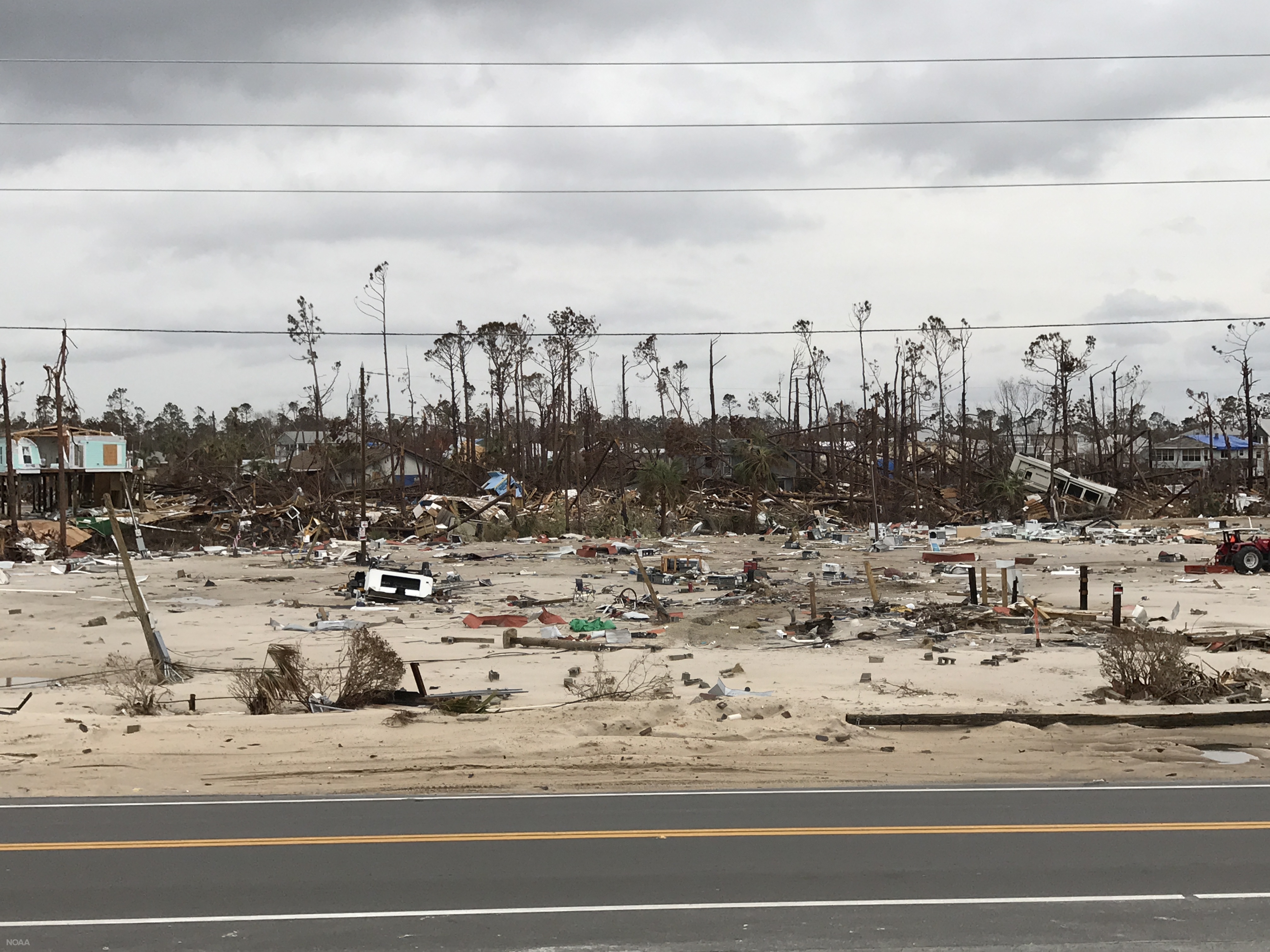
 Mobile home park on the north side of U.S. Highway 98 in Mexico Beach, Florida, washed away by the storm surge and wave impacts of Hurricane Michael. Nov. 2, 2018 (NOAA)
If you were asked to define the word “risk”, what would your response be? What are the first things that come to mind? What questions are you asking? What are some things you would consider to be risky? Risk can take many forms, be it financial, personal injury, or even simple decisions that we all have to make on a daily basis. Consider two simple questions:
- Should I change the tires on my car?
- Should I change the tires on my car today
From a risk perspective, how has the question changed? The answer to the first question is a simple one because it’s general in nature. Yes, the tires should be changed somewhat routinely over the lifetime that you own or lease the car. Question two requires more thought, however, because it narrows the task down to a specific time frame. If your tires were changed recently and are in good shape, then it’s most likely business as usual. If you’re overdue, what are the potential consequences of not having your tires changed? Are you risking personal injury to yourself, your family, or others by not changing them? The risk profile changes based on myriad variables that exist. As this example conveys, the idea of risk is relatively simple in itself but can become complex quickly. Let’s define risk for now as the potential of gaining or losing something of value. That is to say:
Risk = Probability x Consequence
Yes, we threw some math at you, but this concept is relatively easy to grasp. Using the previous example, the overall risk profile is determined by multiplying the probability of a given event by the resulting consequence if that event occurs. So if there is a high chance of an event occurring, or the consequence is severe, then the risk to you would be high. One way to look at risk is by using a risk matrix, as shown below in Figure 1. Your risk increases if the probability of the event goes up or if the consequence of the event goes up.
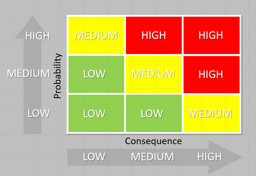
Figure 1. Risk matrix showing different levels of risk based on the probability of an event and the consequence if that event occurs.
The event in our car example is blowing a tire on the interstate, and a potential consequence would be having a fatal accident due to the blown tire. That consequence is so severe that your risk is quite high. But let’s take the example a little further. Risk is further compounded by vulnerability. Let’s consider a new equation:
Risk = Probability x Consequence x Vulnerability
Using the same example, what are variables that could increase the vulnerability, and thus the risk of a fatal accident, in this scenario? Are there kids in the car? What speed is the car travelling? If the tire pops while backing out of the driveway, isn’t that much different than the tire popping while travelling 70 mph down a busy interstate? This is just one of many examples that we all encounter on a daily basis. If there is a consequence to an action you might take, then you are making a risk-based decision.
Risk Perception and Risk Tolerance
There are two other topics related to risk that we should touch on: risk perception and risk tolerance. First, risk perception is the subjective judgement people make about the severity and probability of a risk. Why is this important? Well, there are two main reasons:
- Actual risk usually doesn’t equal perceived risk
- Perceived risk varies from person to person
Why does this complicate matters? When people have to make decisions, it’s important that how they perceive the risk be equal to the actual risk of the event, or at least as close to equal as possible. This is especially true when there is a desired response or action that needs to be taken to protect life and property, as is often the case with weather. We can use a simple example to further understand this. If a tornado is on the ground moving towards a community, the desired action for people living within that community is to seek shelter. In this scenario, the cost of persons within that community not seeking shelter is very high given that their lives are potentially in peril. If people dismiss what that tornado could do to their community (e.g., “tornadoes always pass our city to the south”), then that can be a recipe for disaster, especially when the cost is human lives.
This leads us nicely into risk tolerance. How an individual responds to risk is governed by their risk tolerance, which is unique to both the situation and the person. Risk tolerance is the amount of risk that an individual is willing to accept with respect to a given event occurring. Turning back to the tornado example, let’s consider two hypothetical people that live in the community threatened by the approaching tornado; we’ll name them Sara and Monika. For the sake of example, let’s assume that Sara has a family with two young children and lives in a mobile home. Monika, on the other hand, lives by herself in a well-built house. If Sara and Monika have the same perception of the imposing risk, do these life factors change their respective risk tolerances? In the real world it’s difficult to say, but in this idealized example, let’s assume that it does. Monika does not have anyone in her care and also lives in a home that could withstand stronger winds than Sara’s mobile home. Is Monika’s tolerance for risk higher than Sara’s? It certainly could be, couldn’t it? Again, we understand that assumptions are being made here, but this is simply a hypothetical scenario to demonstrate how risk tolerances may change across individuals and circumstances unique to those individuals. All of this is to say that humans are complicated and risk perceptions and tolerances vary across all of us.
Circling back to the initial equation that we used to define risk, let’s establish a baseline for what the potential consequences are with respect to storm surge by looking at history. Storm surge is the abnormal rise of the ocean produced by a hurricane or tropical storm, and normally dry land near the coast can be flooded by the surge. Historically, about 50% of lives lost in landfalling tropical cyclones in the United States have been due to storm surge (Figure 2):
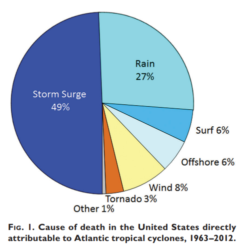
Figure 2. Causes of death in the United States directly attributable to Atlantic tropical cyclones, 1963-2012 (Rappaport 2014).
The mission statement of the National Weather Service charges us to “provide weather, water, and climate data, forecasts and warnings for the protection of life and property and enhancement of the national economy.” There is no clearer way to illustrate what the consequences are in this equation: the loss of human lives. Because the cost here is so high – arguably the highest – our risk tolerance for your safety is extremely low. We have absolutely no appetite for someone losing their life from a weather event. This idea directly informs many of the products that we use to communicate risk prior to and during landfalling storms, and we therefore use near-worst-case scenarios to encapsulate the full envelope of storm surge risk to communities. One life lost during a storm is one life too many. The remainder of this blog post will discuss two such products used by the National Hurricane Center and emergency managers to understand storm surge risk.
MOMs and MEOWs
Can we all agree that “MOMs” are extremely important? Well, yes, those moms are important in our lives, but that holds true for storm surge MOMs as well. Have you ever wondered how officials decide what areas should evacuate ahead of a hurricane? Look no further. MOMs (Maximum of the Maximums) are the rock from which the nation’s storm surge evacuation zones are built upon. MOMs are generated ahead of time. That is to say that these are precomputed maps meant for planning and mitigation purposes well ahead of a landfalling hurricane. In fact, one can view these any time as they are hosted on the National Hurricane Center’s website at https://www.nhc.noaa.gov/nationalsurge/. MOMs are generated by hurricane category (think 1-5) and depict the maximum storm surge height possible across all storm surge attributes. Attributes include things such as forward speed, storm trajectory, and landfall location, just to name a few. Because this product is designed for planning, you can think of the MOM as a worst-case scenario for a given category of a storm. MOMs do have limitations, however. Remember at the beginning of this post we asked the question “should I change the tires on my car?” MOMs are similar to that question because they are general in nature in that they lump all types of hurricanes into a single category. They can tell you what type of storm surge risk you would have from a category 3 hurricane, for example, but they’re not quite as helpful if you know that the category 3 hurricane will be moving toward the west (and not north or northeast for instance).
For this reason, the MOMs have a slightly more refined counterpart – MEOWs (Maximum Envelope of Water). MEOWs are like the second question we asked: “should I change the tires on my car today.” Since we said “today,” we know a little bit more about the actual situation we’re dealing with to make a better-informed decision. Similarly, once a storm or hurricane forms and is within 3–4 days of impacting the coast, we have at least some idea of how strong it could get, how fast it’ll be moving, and in what general direction it’s headed. We are able as forecasters to whittle down the worst-case MOM such that we only consider storms moving toward a particular direction at a particular forward speed — not all directions and forward speeds. Similar to the Maximum of Maximums, a MEOW is a worst-case for storms of a certain strength (for example, Category 3 hurricanes), but it’s more representative of what the storm surge at individual locations could be based on the attributes and forecasts of the active tropical cyclone. At 3 days out, there is still considerable forecast uncertainty, so the MEOW is meant to supplement the MOM, not replace it. As some might say, you can’t go wrong if you always trust your mom. The same adage goes for a hurricane storm surge MOM.
Hurricane Florence
To help us better understand these products, let’s look at how they could have been used in practice during a past landfalling hurricane. Hurricane Florence made landfall along the North Carolina coast on Friday, September 14th of 2018 and presented numerous forecast challenges, as many landfalling tropical cyclones typically do. One benefit of using MOMs and MEOWs to plan, especially at longer lead-times, is that they provide stability in a situation where the forecast of the storm itself can often change quickly from advisory to advisory. Let’s take a look at what Florence’s forecast looked like about 5 days out from an expected landfall. Figure 3 is taken from the official forecast from the National Hurricane Center on September 8th at 11 pm AST.
 Figure 3. NHC five-day forecast track and cone of uncertainty issued for Tropical Storm Florence at 11 PM AST September 8, 2018 (Advisory 39).
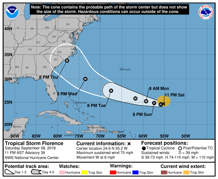
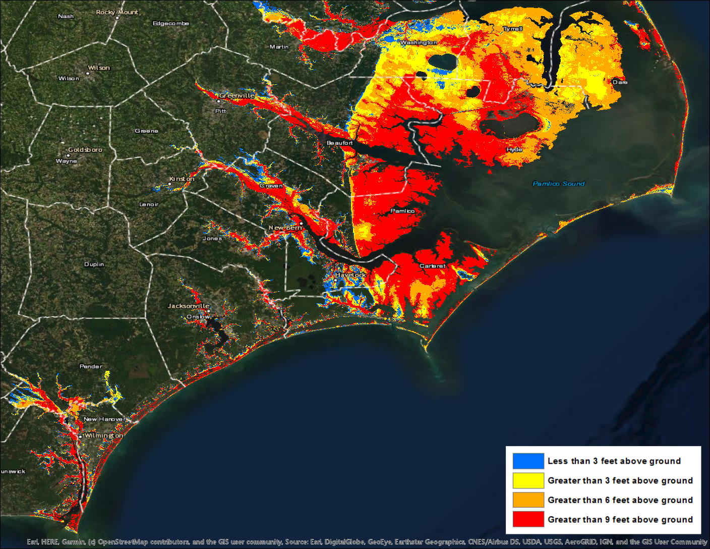
At this point, the information we know is that a potential major hurricane is roughly 5 days away from impacting some portion of the Mid-Atlantic or southeast coast. This is a good point to begin looking at the MOMs. Florence at this point is forecast to be a category 4 hurricane at landfall, so a good rule-of-thumb to follow is to look at a MOM one category higher than the forecast intensity. Let’s take a look at the Category 5 MOM to get an idea of a worst-case storm surge scenario for a portion of the North Carolina coast. You can find that image below in Figure 4.
 Figure 4. Category 5 storm surge Maximum of Maximums (MOM) for portions of eastern North Carolina.

Given how strong Florence could be, it’s no surprise to see potential inundation that would be catastrophic. Remember what we are looking at here and also that this is still a planning tool. This graphic is showing you the worst-case scenario from a Category 5 hurricane. That is to say that these are the highest possible inundations at each individual location for any given storm attribute. We actually shouldn’t expect to see these types of inundation values across the entire area, but given the uncertainties in the storm, all locations in this area should be prepared for these types of inundation values. It would also be prudent to consider looking at other MOMs as well, for context. For example, viewing the Category 3 and 4 MOMs gives context if Florence was to reach the coast at a lower intensity.
Good. Now let’s fast forward by 2 days. We are now 3 days out from a potential landfall. Forecast confidence has increased, but the fine-scale details are still quite blurry regarding the exact location of landfall and how strong Florence will be. But this is when you can begin to turn to the MEOWs. From this point, we can begin to whittle down the MOMs to generate a more realistic potential scenario based on the information currently available. Below in Figure 5 is the forecast from September 10th at 11 pm AST.
 Figure 5. NHC five-day forecast track and cone of uncertainty issued for Hurricane Florence at 11 PM AST September 10, 2018 (Advisory 47).
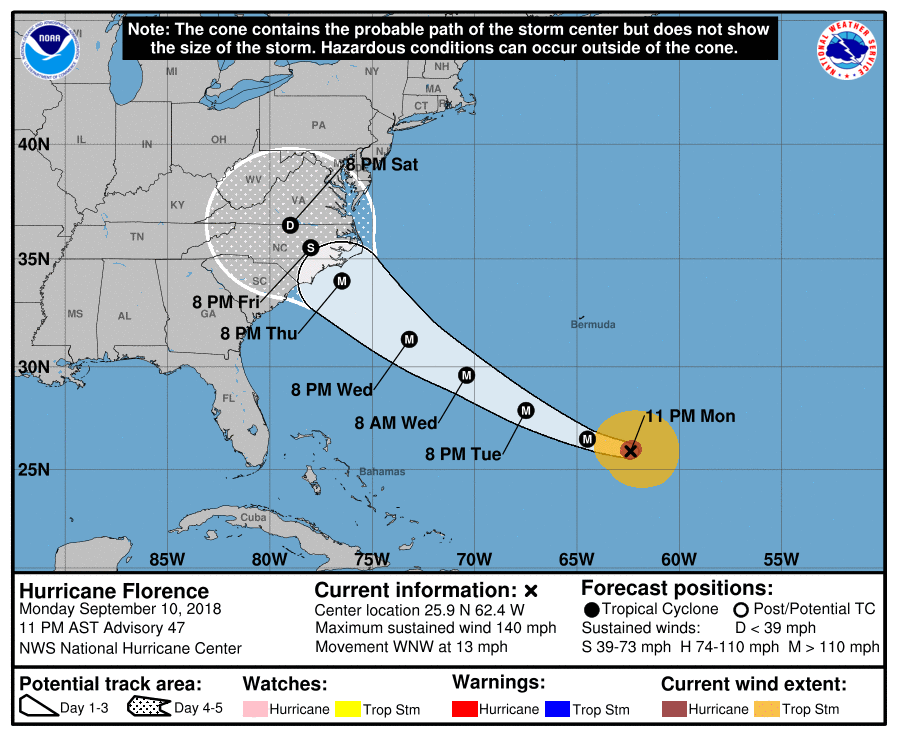
As you can see, there are some updates to the forecast track. The official forecast now calls for Florence to slow down significantly as it approaches the North Carolina coast. Let’s now talk about which MEOWs we should be looking at and explore how we select them. This is an important junction in the forecast because right now we need to evaluate what we do know, what we don’t know, and what we can and cannot rule out. Remember that MEOWs are generated individually for a particular storm category, forward speed, trajectory, and initial tide level. At this point, is there anything that we can rule out in terms of unrealistic directions that Florence could potentially make landfall? It’s ok to acknowledge that there remains some subjectivity here, but it needs to be an informed decision with an understanding that our risk tolerance is low. That being said, let’s go ahead and rule out some storm directions. Since the forecast track in advisory 47 reflects a northwestward trajectory at landfall, we’ll select that direction, as well as the two surrounding it (west-northwest and north-northwest) to account for uncertainty. How about the intensity? The latest forecast still shows Florence reaching the coast as a category 4 hurricane, so we still need to account for the possibility that it makes landfall one category stronger (category 5). Lastly, let’s consider the speed at which Florence is moving and will be moving near its landfall. The tropical cyclone forecast discussion from advisory 47 explicitly mentions that Florence is expected to decrease in forward speed as it approaches the coast:
“After that time [48 hours], a marked decrease in forward speed is likely as another ridge builds over the Great Lakes to the north of Florence.”
This is reflected in the official forecast which slows Florence down to less than 10 mph near the coast. While this certainly complicates the forecast, the beauty of using MEOWs is that it allows you to compensate for this forecast uncertainty. In this case, it’s fair that we could eliminate the MEOW forward speeds of 15, 25 and 35 mph, given forecaster confidence in Florence’s slow down. This leaves us with a forward speed of 5 mph (only a certain set of speeds is actually available to select).
Let’s quickly recap the parameters that we’ve settled on to generate our MEOW:
Intensity: Category 5
Direction/trajectory: Storms that are moving West-Northwest, Northwest, or North-Northwest
Forward Speed: 5 mph
Tide-level: High (this will always be the assumption)
Using those parameters, Figure 6 shows the potential storm surge inundation that could occur across eastern North Carolina:
 Figure 6. Composite storm surge Maximum Envelope of Water (MEOW) over portions of eastern North Carolina for a category 5 hurricane moving west-northwest, northwest, or north-northwest at 5 mph at high tide.
To take this one step further, let’s zoom in around the New Bern, North Carolina, area and do a quick comparison of the category 5 MOM that we initially used 5 days out and compare it to the composite of MEOWs (Figure 7).
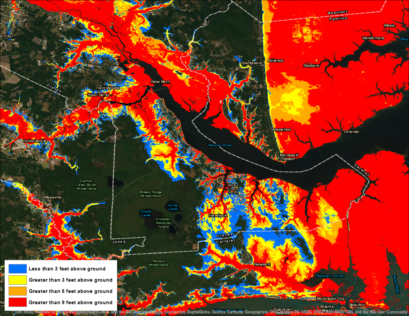
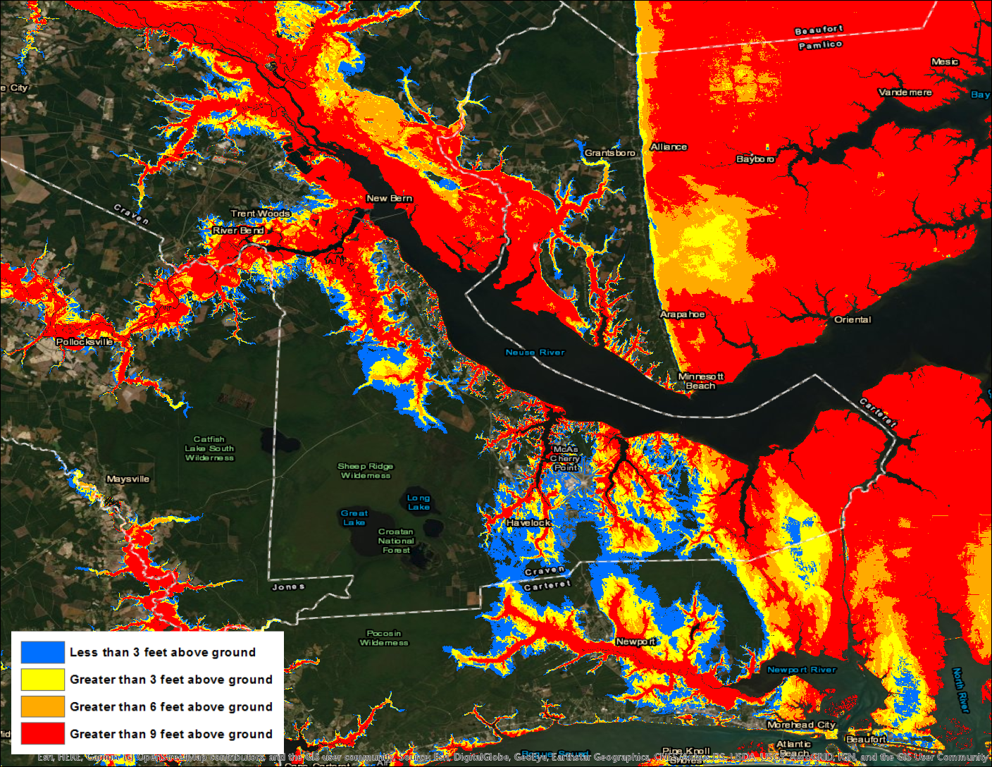
Figure 7. Comparison of MOM (left) and composite MEOW (right) from Figures 4 and 6 above, zoomed in on the New Bern, North Carolina, area.
Remember that at this point in the forecast process, we are looking at synthetic or simulated storms to get an idea of what the near-worst case storm surge inundation could be within an environment characterized by forecast uncertainty that’s very high. What differences do you notice when you compare the two pictures above? Don’t worry–you’re eyes aren’t deceiving you. You probably don’t notice much difference at all. That’s because, unfortunately, slow-moving storms moving in a generally northwestward direction are likely some of the worst types of storms for the New Bern area. Essentially, they’re the storms that are most likely to be causing the storm surge heights you see in the MOM. Our confidence in the hurricane’s forecast has increased since we’re 2 days closer to landfall, but the storm surge risk really hasn’t gone down at all. While that might be a sobering thought, this process allows emergency managers to be as efficient as possible, appropriately assess their risk, and focus on the most at-risk areas. This is a powerful and informative process when used properly!
In the end, while all of eastern North Carolina did not experience the type of storm surge flooding shown in Figure 6 above (which we didn’t expect anyway), some areas did. Areas around New Bern, for instance, had as much as 9 feet of storm surge inundation above ground level (red areas in Figure 8 below). Even though Florence’s peak winds decreased while the storm moved closer to the coast, the MOM and MEOW risk maps accounted for Florence’s increasing size and slow movement (which both contribute to more storm surge) and appropriately prepared emergency managers in the area for a severe storm surge event days before Florence even reached the coast.
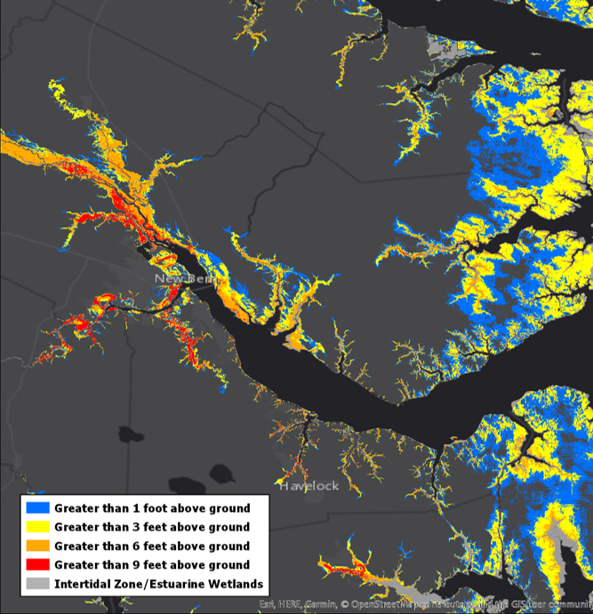
Figure 8. Post-storm model simulation of storm surge inundation caused by Hurricane Florence around the New Bern/Neuse River area of North Carolina.
It’s important to note at this point that MOMs and MEOWs are predominantly used during the period before storm surge or wind-related watches and warnings are in effect for the coast (more than 48 hours before wind or surge is expected to begin). Once we get to within 48 hours when watches or warnings go into effect, another suite of storm surge products–specifically the Potential Storm Surge Flooding Map and the Storm Surge Watch/Warning graphics–become available. These products refine the storm surge risk profile even further because they are based on the characteristics of the actual storm, not on the simulated storms used in MOMs and MEOWs. We plan to create another blog post addressing these products in the near future.
To really bring this home, let’s circle all the way back around to the initial discussion of risk. How does risk tolerance and risk perception affect how these products are used? We know that these products are used by a wide range of people and organizations, all of which have varying tolerances of risk. It is unrealistic to assume that we at the National Hurricane Center could know how these tolerances change across our entire user base. That being said, it is our job to gently guide the decision-making in accordance with our own risk tolerance. Said another way, we work with emergency managers and the Hurricane Liaison Team (HLT) to hopefully bring those risk perceptions more in line with the ACTUAL risk for a given storm. Emergency managers have the resources at their disposal to view MOMs and MEOWs to build out their assessment of risk tailored to their local areas. They possess the intricate knowledge specific to their area which makes them invaluable partners to us at the NHC. During a storm, we sometimes provide advice on types of MOMs and MEOWs to consult to ensure that our partners fully capture a reasonable envelope of risk. These decisions can be stressful, especially when they have to be made in line with a risk tolerance that needs to be low by necessity. Remember what the cost is again here: human lives. It’s imperative that we capture the full breadth of the risk during every storm because the cost of not doing so is immense. We are comfortable accepting that our low risk tolerance can result in some areas not experiencing the potential storm surge that was conveyed prior to a hurricane making landfall. That is, by definition, what having a low tolerance for risk means, but it’s also by design. To us, one life lost is one life too many.
— Taylor Trogdon and Robbie Berg
Reference:
Rappaport, E.N., 2014: Fatalities in the United States from Atlantic Tropical Cyclones: New Data and Interpretation. Bull. Amer. Meteor. Soc., 95, 341–346, https://doi.org/10.1175/BAMS-D-12-00074.1

